Another thirty days of machine learning with Kaggle (Part 2)

Note: This post continues from Part 1, which covered the Kaggle Learn Intro to Deep Learning, Computer Vision, Data Visualization, Intro to AI Ethics and Machine Learning Explainability modules. Part 1 itself continues from my earlier “30 Days of ML” post that covered Python, Intro to Machine Learning and Intermediate Machine Learning.

Data is the foundation of machine learning, and being able to read and manipulate it efficiently is a core skill. While it may not be as sexy as building models and making predictions, data is where it all begins.

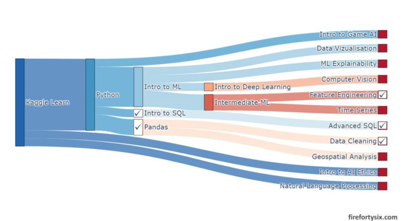
The team at Kaggle clearly acknowledges its importance and has created no less than five data-centric modules, namely Pandas, Intro to SQL, Advanced SQL, Data Cleaning and Feature Engineering.

Before moving on to the more advanced applications of machine learning, I thought that I should spend time building up this foundational skill set in Part 2 of my learning journey with Kaggle Learn.

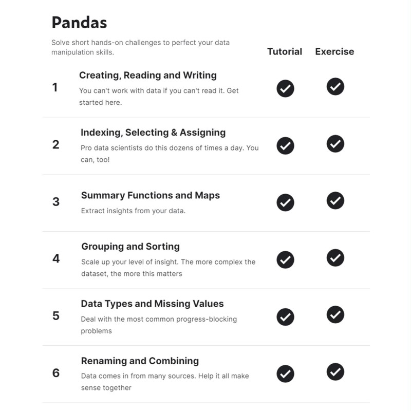
Pandas

The most common and versatile data format used for data science is probably the Pandas dataframe, and this module is a good starting point into the world of data handling.

It starts with the basics of creating a simple dataframe with pd.Dataframe(), reading in a CSV file using pd.read_csv() and writing to a CSV file with df.to_csv() . The module then introduces common actions like indexing, selecting and assigning, as well as useful functions like describe(), unique(), value_counts().

Concepts like the use of map() and apply() to transform data into more useful representations are introduced, and walkthroughs of how to use groupby() and sort_values() are provided. From a practical perspective, it also provides examples of how to deal with missing values and combine different dataframes.

The more I learn about Pandas and Python, the more I like its intuitiveness. For example, one of the indexing exercises asks you to create a smaller dataframe containing all reviews of wines with at least 95 points from Australia or New Zealand from the master wine review dataframe.

This can be done in one easy-to-understand line of code, using the loc[] accessor with an isin() function and & conditional statement. It’s surprisingly close to how I would think about it in my head:

“Locate the reviews where the country is in Australia or New Zealand and where the points are greater or equal to 95.”

And here’s what it actually looks like in Python code:

Most of the other functionality is similarly easy to understand and easy to code. Another example from the grouping exercise asks you to list out all wine reviewers and the average of all the ratings they’ve given. Again, this can be achieved in one line of code by chaining different functions and data elements sequentially.

However, some syntax are a bit more difficult to grasp, at least for me. Especially those that involve lambda functions, such as the example below counting the number of times the words “tropical” and “fruity” appear in the dataset. It should get easier once I use it more frequently.

Intro to SQL

I’ve used SQL (Structured Query Language) in the past, mainly to extract data from corporate databases. I remember not knowing any SQL the first time I had to use it for work, and a colleague helpfully sent me samples of SQL queries that he used on a regular basis.

Whatever I didn’t know, I simply googled and tried it out myself and as long as I didn’t stupidly run any SELECT * FROM ... statements, all was good. That was essentially how I picked up just enough SQL to get my job done.

Reading through the tutorials and doing the exercises gave me a good refresher. Even though I wasn’t familiar with the BigQuery web service used in the module, the SQL statements themselves were pretty standard. The usual suspects were all there: SELECT, FROM, WHERE, GROUP BY, HAVING, COUNT(), ORDER BY, INNER JOIN etc.

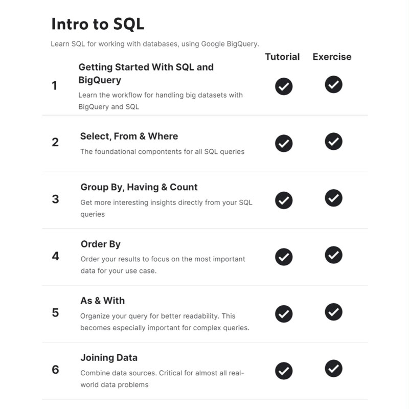
One concept that was new to me was the use of WITH ... AS statements to create a Common Table Expression (CTE). Which is a temporary table created to split queries into a readable chunk, which other queries can then be run on.

See below for an example from the exercises, where the CTE created is RelevantRides that the subsequent SELECT … FROM query is executed against.

Advanced SQL

The topics covered in this module were all new to me, since I’ve never had to run any advanced SQL statements before. It was useful to at least be aware of the more complex SQL queries available, just in case I need to use them in the future.

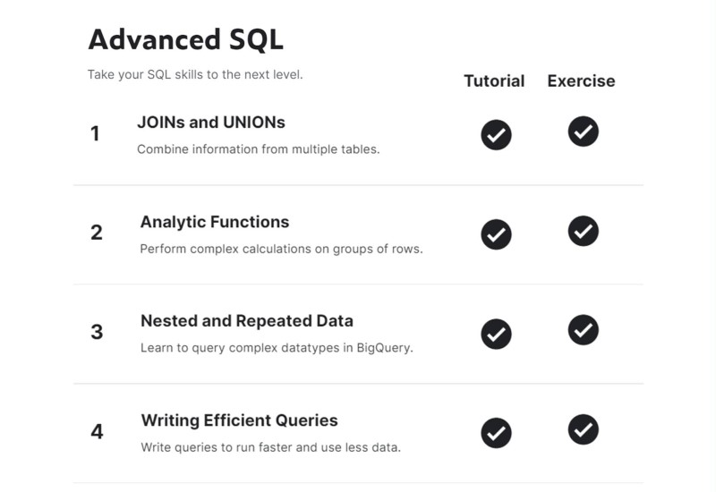
These include the different flavours of JOIN (Inner, Left, Right, Full) and UNION (All, Distinct) queries, as well as various analytic functions for aggregation (AVG(), SUM(), MIN(), MAX(), COUNT()), navigation (FIRST_VALUE(), LAST_VALUE(), LEAD(), LAG()) and numbering (ROW_NUMBER(), RANK()).

More complex data types like nested and repeated data are introduced, and the module ends with strategies on how to write efficient SQL queries, specifically: (i) only select columns you want, (ii) read less data, and (iii) avoid N:N joins.

I’ll definitely have to review the course again, if I ever have to use these advanced features. But for now, it’s sufficient for me to know that they exist.

Data Cleaning

Besides death and taxes, the other certainty in life is that real-world data will be messy. This module covers many practical techniques used to process data before sending it downstream for analysis.

The first hurdle is almost always dealing with missing values, including finding them and then deciding whether to drop them or fill them with reasonable values. This is followed by other tasks such as scaling or normalising data, properly parsing dates, working with different character encodings and handling inconsistent data entries.

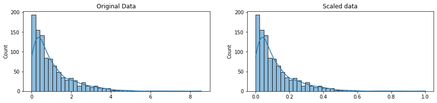
Many useful titbits are scattered throughout the lessons, starting with the distinction between scaling and normalising data.

Scaling changes the range of the data (e.g. 0 to 1) and is used for models that are based on how far apart data points are, such as Support Vector Machines (SVM) or k-Nearest Neighbours (KNN).

Normalising is more intrusive and changes the original distribution of the data to fit the normal distribution. This may be required when using machine learning or statistical techniques that require normally distributed data, such as Linear Discriminant Analysis (LDA) or Gaussian Naive Bayes.

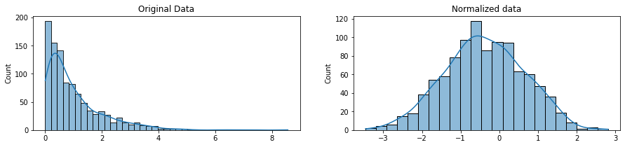
This can be done using Box-Cox Transformation in the scipy.stats package.

Another practical tool covered in the Character Encoding lesson was how to handle errors that arise when using the supposedly straightforward pd.read_csv() function to read in CSV input files.

I encountered this first-hand when I tried doing some geospatial visualisation on global coffee production, and had to read in a relatively simple data file containing names of coffee-producing countries. But the operation failed repeatedly with the following error message:

UnicodeDecodeError: 'utf-8' codec can't decode byte 0xf4 in position 4088: invalid continuation byte

Using the recommended Chardet package, I was able to determine that the character encoding of the data file was not the usual UTF-8 but ISO-8859-1 instead.

Once the correct encoding was ascertained, I was able to read in the file properly by specifying the correct encoding. It turns out that the earlier error message was caused by Côte d'Ivoire, specifically ô which was not a UTF-8 character.

The final lesson on dealing with Inconsistent Data Entry provided a good hands-on exercise on how to use the FuzzyWuzzy (cute name, right?) package to identify strings that are close, but not identical, to each other. When these similar strings are read in, they appear as different data points when they should be considered as the same instead.

Again, I was able to apply this newly acquired knowledge in my geospatial visualisation, by generating fuzzy matches for inconsistent country names between the two datasets I was using. It wasn’t 100% foolproof, but it helped to significantly reduce the time (and grief!) on data cleaning.

It always feels good whenever I get to use what I’ve learnt to fix a practical problem. From that perspective, completing the Data Cleaning module was very rewarding indeed.

Feature Engineering

Feature engineering is not quite data processing nor is it model building per-se, but sits between them in the data science workflow. Objectives include: (i) improving a model’s predictive performance, (ii) reducing computation or data needs, and (iii) improving interpretability of results.

The first tutorial provides a good high-level overview: “the goal of feature engineering is to make the data better suited to the problem at hand.”

Over the course of the lessons, I learnt how to:

• determine which features are the most important with mutual information
• invent new features in several real-world problem domains
• create segmentation features with k-means clustering
• decompose a dataset’s variation into features with principal component analysis
• encode high-cardinality categoricals with a target encoding

The tutorials and exercises were content-rich and used many packages, including sklearn.feature_selection.mutual_info_regression, sklearn.cluster.KMeans, sklearn.decomposition.PCA and category_encoders.MEstimateEncoder. They were definitely worth the effort going through.

Part 3

After finishing all the data-centric modules, the final leg of my Kaggle Learn journey was next. Covering the more application-focused Geospatial Analysis, Intro to Game AI and Reinforcement Learning, Natural Language Processing and Time Series.

Tune in next week for the final episode!