After completing Alexis Cook’s very useful Titanic Tutorial, I couldn’t help myself and spent a couple of days hacking around to try and improve my score without going through the usual data science workflow of EDA, feature engineering, model selection, hyperparameter tuning and train/test iterations.
I know it’s not the proper way of doing data science, but like I said, I just couldn’t help myself.
The Titantic Tutorial provided two possible models: Gender Submission and Random Forest, which I will label as Mark 01 and Mark 02, that scored 0.76555 and 0.77511 respectively.
Given that I had a ready notebook to play with, I decided to make small adjustments to see how they would change the score. Changes were made along two paths: (i) changing the input features and filling missing data, and (ii) changing the machine learning model.
Modifications
Here’s what I tried:
- Mark 01: Download and submit gender_submission.csv from Titanic Tutorial
i.e. Features = Sex; Model = All women survived, all men died - Mark 02: Copy/paste Python code from Titanic Tutorial
i.e. Features = Sex, Pclass, SibSp, Parch; Model = Random Forest (max_iter=100, depth=5) - Mark 03: Extend features by adding Age, with missing data filled using mean of available data
i.e. Features = Sex, Pclass, SibSp, Parch, Age (fill blanks with mean); Model = Random Forest (n_estimators=100, max_depth=5) - Mark 04: Extend features by adding Embarked
i.e. Features = Sex, Pclass, SibSp, Parch, Age (fill blanks with mean), Embarked; Model = Random Forest (n_estimators=100, max_depth=5) - Mark 05: Tweak Random Forest model by increasing number of trees and removing cap on depth
i.e. Features = Sex, Pclass, SibSp, Parch, Age (fill blanks with mean), Embarked; Model = Random Forest (n_estimators=1000, max_depth=None) - Mark 06: Try Logistic Regression model
i.e. Features = Sex, Pclass, SibSp, Parch, Age (fill blanks with mean), Embarked; Model = Logistic Regression (max_iteration=1000) - Mark 07: Try k-Nearest Neighbour (kNN) model
i.e. Features = Sex, Pclass, SibSp, Parch, Age (fill blanks with mean), Embarked; Model = k-Nearest Neighbour (n_neighbours=5) - Mark 08: Try Ensemble model using Mark 05, 06 and 07
i.e. Features = Sex, Pclass, SibSp, Parch, Age (fill blanks with mean), Embarked; Model = Ensemble of Mark 05, 06, 07 (voting=’hard’) - Mark 09: Change Age missing data filling approach to mean of each Name_Title/Pclass combination, where Name_Title (Mr, Miss, Master etc) was extracted from Name; and reverting back to Random Forest model from Mark 03
i.e. Features = Sex, Pclass, SibSp, Parch, Age (fill blanks with mean of Name_Title/Pclass combo), Embarked; Model = Random Forest (n_estimators=100, max_depth=5) - Mark 10: Try Logistic Regression model
i.e. Features = Sex, Pclass, SibSp, Parch, Age (fill blanks with mean of Name_Title/Pclass combo), Embarked; Model = Logistic Regression (max_iteration=1000) - Mark 11: Try k-Nearest Neighbour model using 10 neighbours
i.e. Features = Sex, Pclass, SibSp, Parch, Age (fill blanks with mean of Name_Title/Pclass combo), Embarked; Model = k-Nearest Neighbour (n_neighbours=10) - Mark 12: Try Ensemble model using Mark 09, 10, 11
i.e. Features = Sex, Pclass, SibSp, Parch, Age (fill blanks with mean of Name_Title/Pclass combo), Embarked; Model = Ensemble of Mark 09, 10, 11 (voting=’hard’)
It sounds like a long list of attempts, but given that each successive try was a tweak of the earlier one, the process was basically a repetition of copy-paste-tweak-check-save-submit to get a new score.
This didn’t take much time, except that I’m new to all this and had to pick up some simple Python and scikit-learn syntax along the way, courtesy of Google and stackoverflow.com.
Yes, I know that I should invest some time to pick up Python properly, and I plan to do that soon, but I managed to learn just enough to get the job done. Oh, and since Kaggle restricts the number of submissions to 10 per 24-hour cycle, I had to do this over two days.
Code Snippets
My complete Jupyter notebook is available on Kaggle, and if you’re interested to run the code, you’ll have to create a Kaggle account to fork a copy and then run it inside Kaggle. But if you’re just keen on looking at parts of the code, below are some code snippets.
Mark 04 (Random Forest)
Note that this code snippet uses fillna() to fill in missing Age data using the average of all existing Age data. It also uses get_dummies() to convert categorical data into numerical form by using one-hot encoding.
# Mark 04
# Extend features by adding Embarked
# Features = Sex, Pclass, SibSp, Parch, Age (fill blanks with mean), Embarked

# Model = Random Forest (n_estimators=100, max_depth=5)
from sklearn.ensemble import RandomForestClassifier

y = train_data["Survived"]

features = ["Pclass", "Sex", "SibSp", "Parch", "Age", "Embarked"]
X = pd.get_dummies(train_data[features])
X_test = pd.get_dummies(test_data[features])

X.Age.fillna(X.Age.mean(), inplace=True) # Fill missing values in Age with mean value
X_test.Age.fillna(X_test.Age.mean(), inplace=True)

model = RandomForestClassifier(n_estimators=100, max_depth=5, random_state=1)
model.fit(X, y)
predictions = model.predict(X_test)

output = pd.DataFrame({'PassengerId': test_data.PassengerId, 'Survived': predictions})
output.to_csv('my_submission.csv', index=False)
print("Your submission was successfully saved!")
Logistic Regression
from sklearn.linear_model import LogisticRegression
model = LogisticRegression(max_iter=1000)
model.fit(X, y)
predictions = model.predict(X_test)
k Nearest Neighbours (kNN)
from sklearn.neighbors import KNeighborsClassifier
model = KNeighborsClassifier(n_neighbors=5)
model.fit(X, y)
predictions = model.predict(X_test)
Ensemble Model
from sklearn.ensemble import RandomForestClassifier
model_rf = RandomForestClassifier(n_estimators=100, max_depth=5, random_state=1)
model_rf.fit(X, y)

from sklearn.linear_model import LogisticRegression
model_lr = LogisticRegression(max_iter=1000)
model_lr.fit(X, y)

from sklearn.neighbors import KNeighborsClassifier
model_knn = KNeighborsClassifier(n_neighbors=5)
model_knn.fit(X, y)

from sklearn.ensemble import VotingClassifier
estimators =[('rf', model_rf), ('lr', model_lr), ('knn', model_knn)]
ensemble = VotingClassifier(estimators, voting='hard') # 'hard' = majority vote
ensemble.fit(X, y)

predictions = ensemble.predict(X_test)
Extract Name_Title, Name_Last, Name_First from Name field
One example of Name data is “Braund, Mr. Owen Harris” and so I used the “,” and “.” delimiters to progressively split it into Name_Last = “Braund”, Name_Title = “Mr” and Name_First = “Owen Harris”.
There are definitely more elegant ways of doing this, including the use of regular expressions (regex), but this was what I could do with my current rudimentary Python skills and Googling. It isn’t pretty, but it works.
# Split Name into Name_First, Name_Title, Name_Last
names_train = train_data[['Name']].copy()
names_train [['Name_Last', 'Name_Temp']] = names_train['Name'].str.split(',', expand=True)
names_train [['Name_Title', 'Name_First']] = names_train['Name_Temp'].str.split('.', n=1, expand=True)
names_train = names_train.drop('Name_Temp', 1)
Fill missing Age data with average of Name_Title and Pclass combination
Using the assumptions that (i) Name_Title can help distinguish between, for example, a male adult (Mr) and child (Master), and (ii) that people who could afford a higher ticket class (Pclass) are generally older, I improved on the missing Age data-filling logic by using a more granular average of the Name_Title and Pclass combination. Any combination that is still missing would fall back on the simple average of all.
X['Name_Title'] = names_train['Name_Title'] # Append Name_Title to train_data

X['Age'] = X['Age'].fillna(X.groupby(['Name_Title', 'Pclass'])['Age'].transform('mean')) # Fill missing Age with mean of Name_Title/Pclass combination e.g. Mr/3
X['Age'] = X['Age'].fillna(X['Age'].mean()) # Fill any remaining blanks with simple mean of all Ages

X = X.drop('Name_Title', 1) # Drop Name_Title as only used for filling missing Age, not for modelling
Results
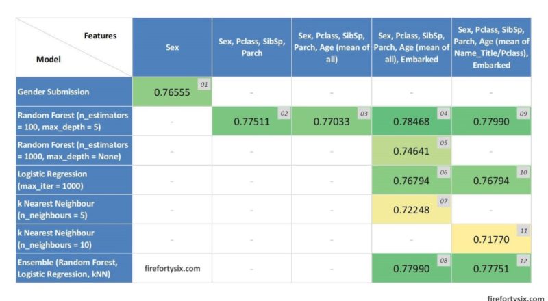
Here’s a visual summary of all the submitted test scores from Mark 01 to 12, in a table listing the features and models used. The heatmap highlights the lowest score as yellow, the highest as dark green and the rest as shades in-between.

Some quick observations:
- Adding features seems to improve scores more than using different models. Although it could be that the Random Forest model in Titanic Tutorial was already quite good, better than Logistic Regression or kNN.
- Changing the filling method of missing Age data from a simple mean of all available vs a slightly more involved mean of Name_Title/Pclass combo didn’t improve scores, in fact it made them slightly worse.
- Using an Ensemble model did not improve scores of the best performing Random Forest model. Again, it could be that the Random Forest model was much better than the other two other models that using an ensemble made final predictions worse.
- It seems that using a fairly complex Random Forest model with many features (Mark 04) didn’t really improve the super simple “all women survive, all men die” model (Mark 01) by a lot. The score only increased by a small 2.5%, showing that sometimes, simple is best.
While this hacking around is clearly not the right way to approach a data science problem, it did help scratch my itch of quickly trying different settings and seeing how they performed vs each other. I hope you found these results entertaining at least.
Now, back to doing things “right” and starting from scratch with EDA in a new notebook.